Basic principles of the coarse-graining procedure

MagiC is a software package designed to perform tasks of multiscale structure based coarse graining in molecular simulations. This is done by extracting radial distribution functions (RDF) and other structural information from a high resolution (fine grained) simulation of the system of interest (reference system), and then to generate effective potentials which reproduce these RDFs in a coarse-grain model by means of the inverse Monte-Carlo method or Iterative Boltzmann inversion method. Such potentials can be further used for large scale simulation.

In general systematic coarse graining can be considered as a multi-stage process which leads from a high resolution system description to the low resolution one (see figure 1).

Figure 1: Systematic Coarse-Graining with MagiC: General outline. Blue rectangles denote input/output data; purple rectangles denote data processing procedures. Optional input data and use of external software are marked with dashed frame.

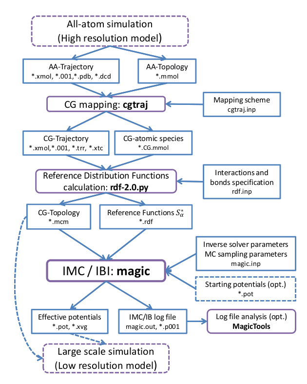Each step (shown in purple) uses results of the preceding stage output as an input (input/output is shown in blue), and additional input provided by user (rightmost blue blocks).

Five stages can be distinguished:

1. The system of interest is simulated at high resolution, e.g. using Molecular Dynamics simulation with all-atom (AA) force field. Such a simulation results in atomistic (AA) trajectory which is supposed to sample the atomistic system well enough. This simulation can be performed by any suitable external molecular dynamics (or Monte Carlo) software.

2. A coarse-grained (CG) trajectory is generated from the atomistic trajectory obtaned during the first stage. This is performed by utility [cgtraj]cgtraj which is a part of MagiC. It converts AA-trajectory into CG-trajectory, using a user provided mapping scheme which states the correspondence between atomistic and CG representations for every molecular type. This stage results in a coarse-grained trajectory and mass/charge properties of CG-beads stored in molecular description files (.mmol).

3. Structural reference distribution functions are calculated by the utility [rdf]rdf.py. Since every distribution function corresponds to a specific interaction, definitions which interactions and bonds are present in the CG system are defined at this stage.

4. The inverse problem is solved by the Inverse Monte Carlo or Iterative Boltzmann Inversion methods. This is the key stage, which is done by a core of the package which is called [magic]magic core. During this stage, effective potentials between CG sites are iteratively refined to fit the RDFs obtained in atomistic simulations. Also, an extended log-file is generted which reports details of every IMC/IBI iteration. The files can be analyzed by a set of post-processing tools [MagicTools]MagicTools, which allow to plot the convergence rate, effective potentials from each iteration, potential corrections at each iteration, intermediate RDFs, etc.

5. Once the effective potentials reproducing the reference RDFs with required precision are obtained, they can be exported by MagicTools to an external MD software and used for further simulations of the large scale CG system. At the moment export to GROMACS format is provided, extentions to other mesoscale simulation software accepting tabulated potentuals can be made relatively straightforwardly.

Since MagiC is implemented as a set of separate programs, it is possible to perform different tasks on different computers, for example run the most time-consuming part of the calculations, inversion of RDFs (stage 4), on a high performance cluster, and perform analysis on a local desktop computer.