In general systematic coarse-graining can be considered as a multi-stage process which leads from
a high-resolution model to the low-resolution one (see figure 1).
Figure 1:
Systematic Coarse-Graining with MagiC: General outline.
Blue rectangles denote input/output data; purple rectangles denote data processing procedures.
Optional input data and use of external software are marked with dashed frame.
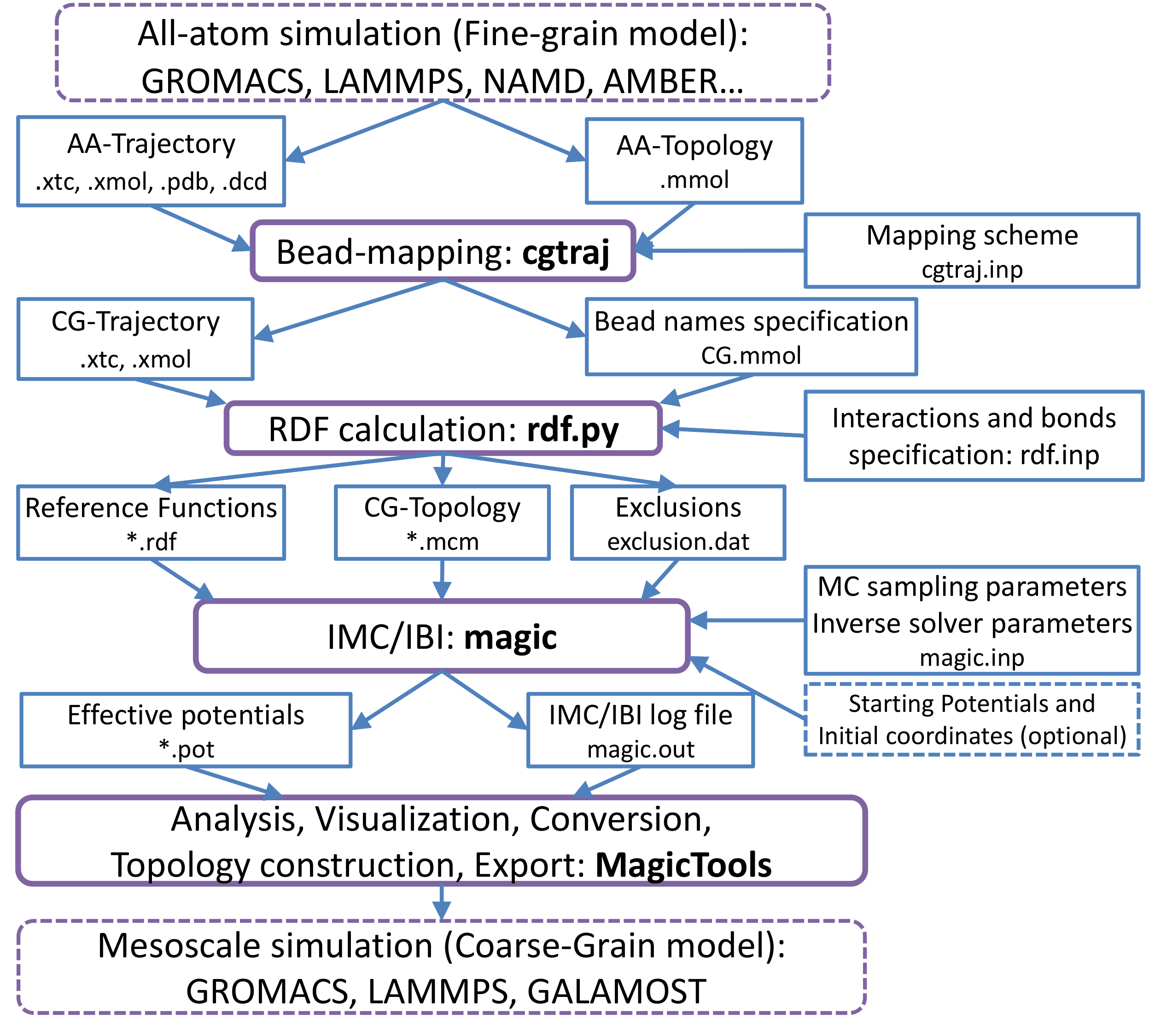 |
Each step (shown in purple) uses results of the preceding stage output as an input (input/output
is shown in blue), and additional input provided by user (rightmost blue blocks).
Six stages can be distinguished:
- The system of interest is simulated at high resolution, e.g. using Molecular Dynamics
with all-atom (AA) force field. Such simulation results in AA trajectory
which is supposed to sample the atomistic system well enough. This simulation can be performed by
any suitable external molecular dynamics (or Monte Carlo) software.
- A coarse-grained (CG) trajectory is generated from the atomistic trajectory
obtaned during the first stage. This is performed by utility cgtraj
which is a part of MagiC. It converts AA-trajectory into CG-trajectory, using a user provided
mapping scheme which states the correspondence between atomistic and CG representations
for every molecular type. This stage results in the coarse-grained trajectory and mass/charge
properties of CG-beads stored in molecular description files (
.CG.mmol).
- Structural reference distribution functions are calculated by the utility rdf.py.
Since every distribution function will correspond to an effective potential, at this stage we define all interactions in the CG-model. This includes bead types assignment, definition of pairwise and angle-bending bonds. Based on the bond connectivity, the list of sites excluded from non-bonded interactions is generated.
As the result of this stage user gets RDFs containing file (*.rdf), CG molecular topologies (*.mcm) and exclusion definitions (exclusion.dat)
- The inverse problem is solved by the Inverse Monte Carlo or Iterative Boltzmann Inversion methods.
This is the key stage, which is done by a core of the package which is called
magic core. During this stage, effective potentials between CG sites are
iteratively refined to fit the reference RDFs. An extended log-file reports details of every IMC/IBI iteration.
- Model analysis by the set of post-processing tools MagicTools.
It allows to plot the convergence rate, effective potentials from each iteration,
potential corrections at each iteration, intermediate RDFs, etc.
- Once the effective potentials reproducing the reference RDFs with required precision are
obtained, they can be exported by MagicTools to an external MD software and used for
further simulations of the large scale CG system. At present it supports GROMACS, LAMMPS and GALAMOST, however, extensions to other MD simulation software accepting tabulated potentials
can be made easily and smoothly.
Since MagiC is implemented as a set of separate programs, it is possible to perform different
tasks at different locations, for example run the most time-consuming part of the calculations,
inversion of RDFs (stage 4), on a high performance cluster, and perform analysis on a
local desktop computer.