Potential export procedure details

The export is rather complex process, here we give some details about how it is done.

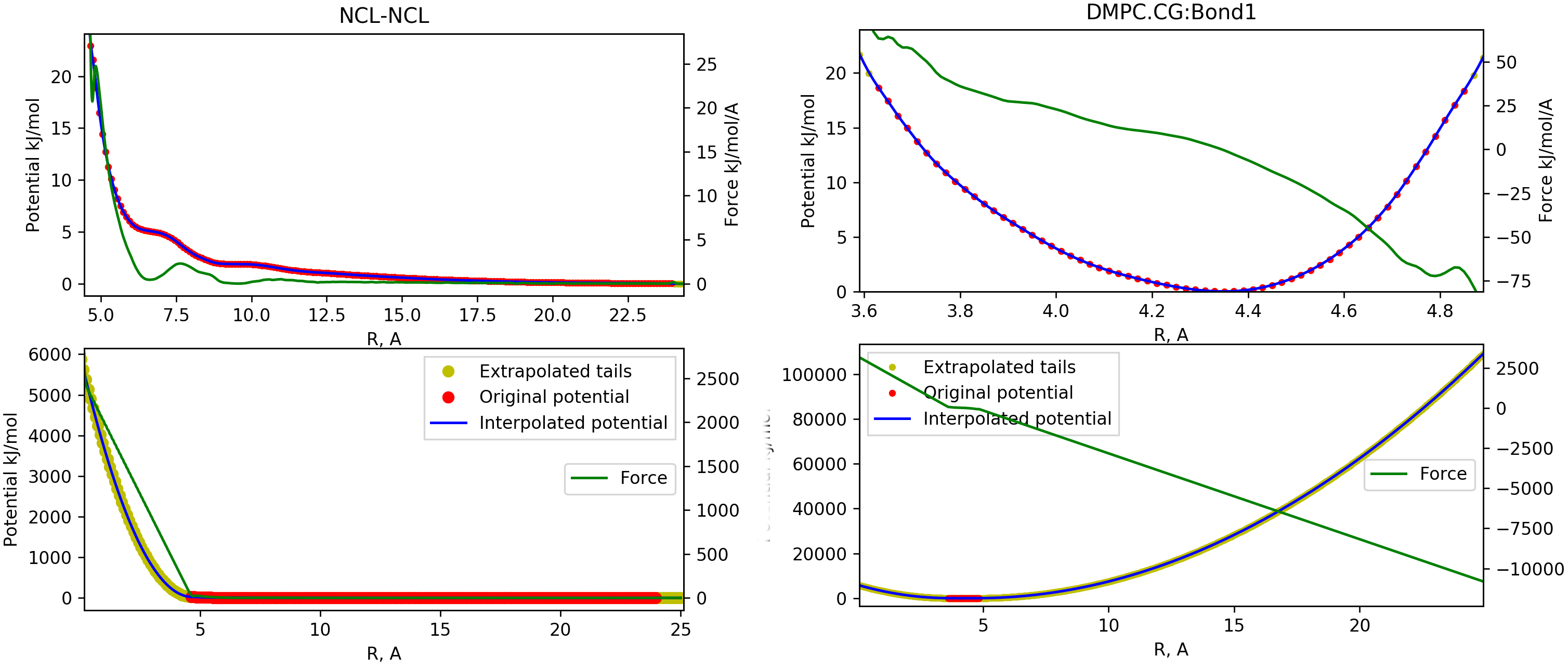
The molecular dynamics simulation heavily relies on quality of the tabulated potentials, i.e. the potential and force should be smooth and do not have discontinuities at the whole range $[0-r_{cutoff}]$.

The Monte Carlo approach, however, is much more tolerant to the potential quality, the potential obtained in the inverse process is defined on a relatively sparse grid, may have kinks, and is defined at the limited range $[r_{min}:r_{max}]$.

Thus the short-range potential, which is generated by the MagiC core, have to be extrapolated both at the left-hand side and at the right hand side. Moreover, it is desirable to interpolate the potential to a higher grid density and also make it smooth to avoid numerical instabilities in force calculation.

In MagiC implementation, the left side extension represents a strongly repulsive core, and it is approximated by $U^{left}(r)=ar^2+br+U_{max}$ on the range $[0:r_{min}]$, and coefficients $a$ and $b$ are chosen to provide continuity of $\frac{d}{dr}U(r)$ at $r=r_{min}$.

The right side extension may differ, depending on the type of the potential. Non-bonded potentials should smoothly decay to zero when $r_{max}< r<r_{cutoff}$, this is achieved by using this expression:

$$U^{right}_{short\,range}(r)=U(r_{max})\cdot\exp[{-10\frac{(r-r_{max})}{r_{cutoff}-r_{max}}}]$$ (7)

Here 10 is some predefined coefficient, $r_{cutoff}$ is the range of the resulting potential table as required by the MD Engine.

Angle-bending potentials should also decay to zero at $\phi=180^{\circ}$ which is implemented by:

$$U^{right}_{angle}(\phi)=U(\phi_{max})\cdot\exp[{-100\frac{(\phi-\phi_{max})}{180^{\circ}-\phi_{max}}}]$$ (8)

Pairwise bond potentials should have an attractive wall at the right side, which is approximated by harmonic wall in the same way as the repulsive wall at the left side:

$$U^{right}_{pair\,bond}(r)=ar^2+br+U_{max}$$ (9)

coefficients $a$ and $b$ are chosen to provide continuity of $\frac{d}{dr}U(r)$ at $r=r_{max}$.

Once the original potential has been extended, all intermediate points are interpolated to a denser and smoother grid. Number of nodes in such grid is defined by parameter npoints.

The interpolation can be made either by SciPy radial basis function interpolation, or Gaussian smoothing, e.g. interpolated values are calculated as a exponential-weight average:

$$U^{new}(r)=\frac{1}{Z(r)}\sum_{r_i=r_{min}}^{r_{max}}{U^{orig}(r_i)\cdot\exp{\frac{-(r-r_i)^2}{2\sigma^2}}}$$ (10)

$$Z(r)=\sum_{r_i=r_{min}}^{r_{max}}{\exp{\frac{-(r-r_i)^2}{2\sigma^2}}}$$ (11)

where sigma defines how broad is the averaging. By default $\sigma$ is half resolution of the original table. The first of the interpolation methods provides smoother force, however may be subject to artifacts at large distances.

If interpol=False, the original grid will be kept.

Once the interpolation is done, each resulting potential and force based on it are written to table-files in the format corresponding to the desired MD engine. For LAMMPS it is *.table-file as described here and here.

For GROMACS, it is *.xvg format described here. Forces can be suppressed by setting noforce=True, then zeros will be written to the file. In such case GROMACS should automatically calculate forces from a given potential.

For GALAMOST it is *.dat format, which has no description on the web, so we recommend to take one of our Tutorials to see an example there.

Each table file is named by the name and the type of the corresponding potential.

In order to control the results, each original potential, the extrapolated part and the interpolated potential are plotted together, so the user can visually inspect the result and check for artifacts, fluctuations and other numerical issues which may occur. The example of such plot is shown on figure

Figure: Example of potential exporting control plots. Left side - Non-bonded potential, Right side - pairwise bond potential. Upper plots display the initial range $[r_{min}:r_{max}]$, lower plots display the full range $[0-r_{cutoff}]$ (after the extension). Red circles denote original potential values, yellow circles show extended values (both defined on sparse grid). Blue line shows interpolated potential defined on dense grid, and green line shows the calculated force.